If you are using the dot grid method to assess tree canopy cover, how many dots do you need to count? Unfortunately, there is no single answer to this question, but you can calculate the minimum sample size of dots required for a given application if you have some basic information about the population. Several basic principles apply when determining the necessary sample size. First, the reliability of the canopy cover estimate will increase as the dot density increases, but the increase in statistical power begins to plateau at high sample sizes. This effect is evident when power is plotted against sample size (Graph 3-1). Larger sample sizes are needed when making comparisons between similar canopy cover levels (e.g., comparing tree cover changes over time due to natural mortality) than when comparing widely different canopy levels (e.g., comparing tree cover in residential and industrial areas) (Graph 3-2). Also, the sample size needed to detect a difference of a given magnitude (e.g., 10%) increases as the percent cover approaches 50% (Graph 3-3).
The upshot of this is that almost any application will require a count of at least 300-400 dots. If you need higher precision or if you need to differentiate between levels of canopy that are close to 50%, the minimum dot count will be closer to 500, and higher numbers would be preferable.
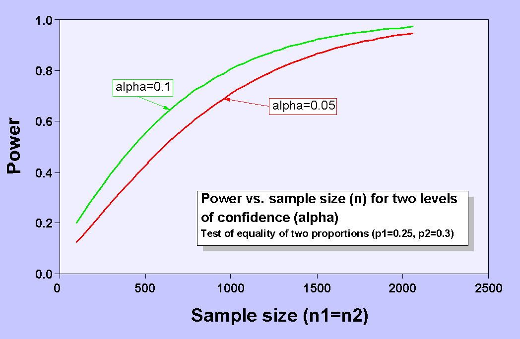
The graph below shows the general shape of a sample size power curve. All of the curves shown on this page are based on the formula for a test comparing two proportions (p1 and p2). Power is plotted on the vertical axis and sample size is on the horizontal axis. You can see from the graph that power increases with increasing sample size, but the slope of the curve decreases progressively as sample size increases, that is, you reach a point of diminishing returns. For example, at alpha (or confidence level) =0.05, sample size needs to be increased by about 200 to increase the power from 0.6 to 0.7, but it needs to be increased by about 450 to increase the power from 0.8 to 0.9. The graph below shows curves for two different levels of alpha. For a given level of power, a larger sample size is needed to obtain a higher confidence level.
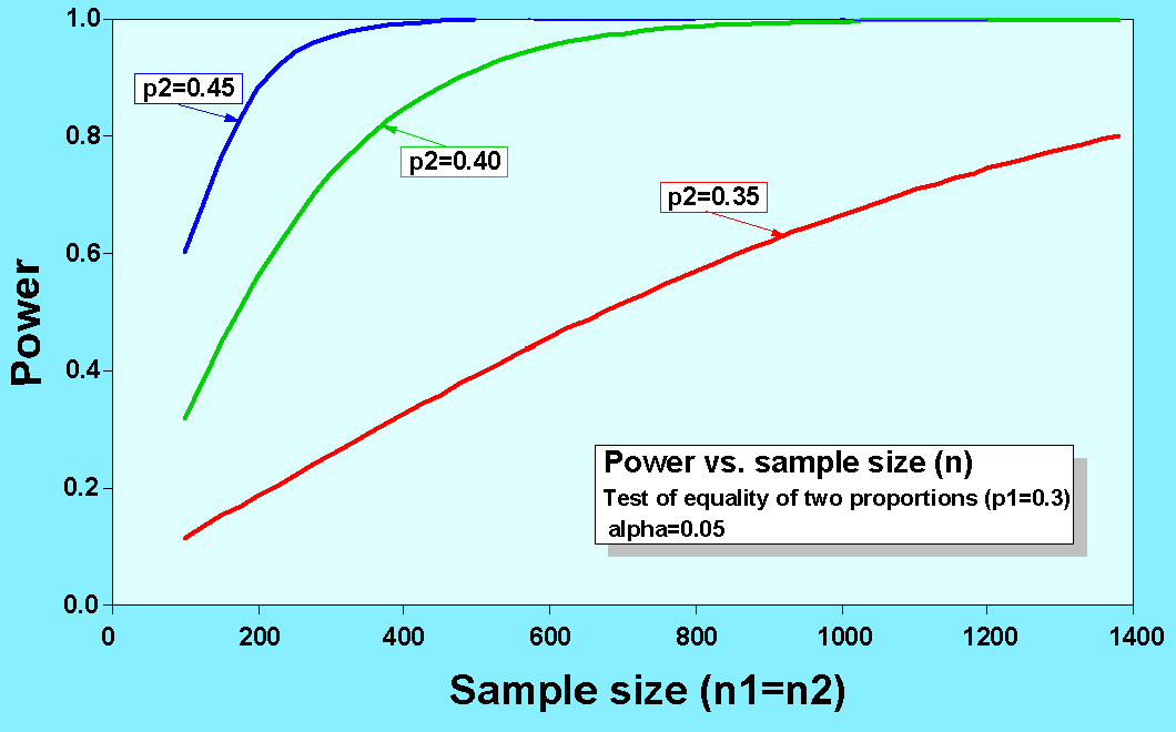
As illustrated in the graph below, sample size must increase to detect relatively
small differences at a given level of power
and confidence. In the example shown,
at alpha=0.05 and power=0.8, a sample size of about 170 dots will suffice for
detecting the difference between 30% and 45% canopy cover, but a sample size
of 1400 dots is needed to detect a real difference between 30% and 35% canopy
cover. Looking at this effect another way, at a sample size of 400 dots, a statistical
difference between 30% and 45% canopy will be detected more than 99 times out
of 100; a difference between 30% and 40% canopy will be detected about 85 times
out of 100, but a difference between 30% and 35% canopy will only be detected
about 33 times out of 100.
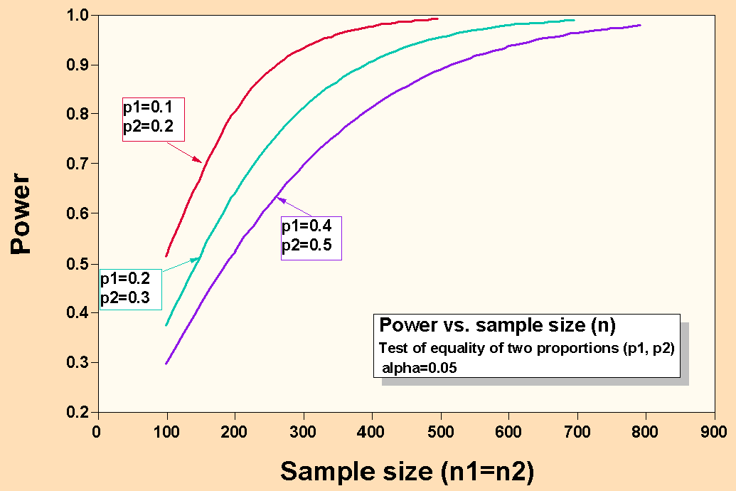
In the graph below, the magnitude of the difference to be detected is the same
for all three curves (0.1). You can see that progressively larger sample sizes
are needed to obtain a given level of power
as the proportions approach 0.5. This relationship is symmetrical around the
center of the range (0.5). Thus, the curve for the pair p1=0.9 and p2=0.8 is
the same as the curve for the pair p1=0.1 and p2=0.2.